In my previous post, we discussed the signal — the functional form. We saw how getting the shape of a relationship wrong (for example, assuming a straight line when the true effect is curved) can lead to biased policy estimates. Today, we turn to the other half of the story: the noise or the stochastic component of a model.
In this post, we will unpack what this “noise” really means and why the specific distributional assumptions we make about it — such as assuming that errors are “Normal” — are not just academic details. They quietly, but fundamentally, shape the risk, confidence, and reliability behind every major decision.
What is the Stochastic Component?
Every statistical model has two parts: one that captures what we can explain (the Signal), and another that simply acknowledges what we can’t. The part we can’t explain—the leftover, unavoidable randomness—is what statisticians call the stochastic component, or more simply, the error term (ϵ).
No matter how sophisticated our model is, there will always be factors we miss, measurement errors we can’t avoid, and inherent randomness we can’t control. This unexplainable part is not a flaw. It is a recognition that data, and the real world it represents, are never perfectly predictable.
What is a Distribution Assumption?
When we make a distributional assumption, we are essentially describing the shape of that randomness—a kind of blueprint for the noise. For example, are the errors usually small and balanced around zero, or do large, surprising deviations occur more often than we expect?
Think of this as a target practice. Getting the functional form right is about aiming at the correct spot on the target. If you assume a straight line when the true effect bends, your aim is off. The stochastic component, however, describes the scattering pattern of your shots. When the pattern is tight and centered, your aim is precise; when it is wide or lopsided, your precision falters.
Assuming the wrong distribution is like overestimating your own accuracy. You might hit the bullseye once and claim success, but your overall precision — your confidence in that hit — would be misleading. The stochastic component doesn’t change where your dart lands on average, but it determines how confident you should be in that landing spot.
What are Some Common Distributions?
Every statistical model must assume how its errors behave. This assumption—the error distribution—acts like the model’s mental image of how unpredictable the world truly is. Some models imagine the noise as gentle and symmetric; others account for lopsided patterns or a surprising tendency toward big deviations.
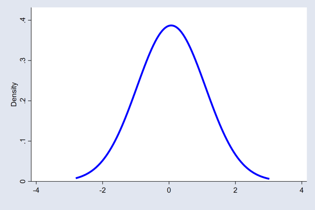
The Normal distribution is the one most people recognize. It assumes the errors are continuous, symmetric, and mostly small, with extreme errors being very rare. It’s the model’s way of saying, “Most of the time, I’m close to the mark, and big misses hardly ever happen.” This works well for many economic, social, and behavioral data, where variation tends to be moderate and balanced (see figure 1).
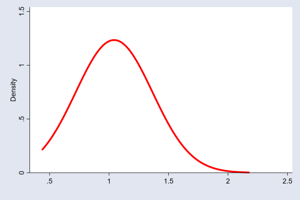
But not all noise behaves so neatly. When errors are skewed, large deviations occur more often on one side than the other. In such cases, the Log-normal Distribution is often a better blueprint. It assumes errors are always non-negative and usually small but occasionally can be very large. This is the error structure for variables like wealth or income, where you can’t have negative values, but a few extremely high values stretch the right-hand side, making the overall uncertainty lopsided (see figure 2).
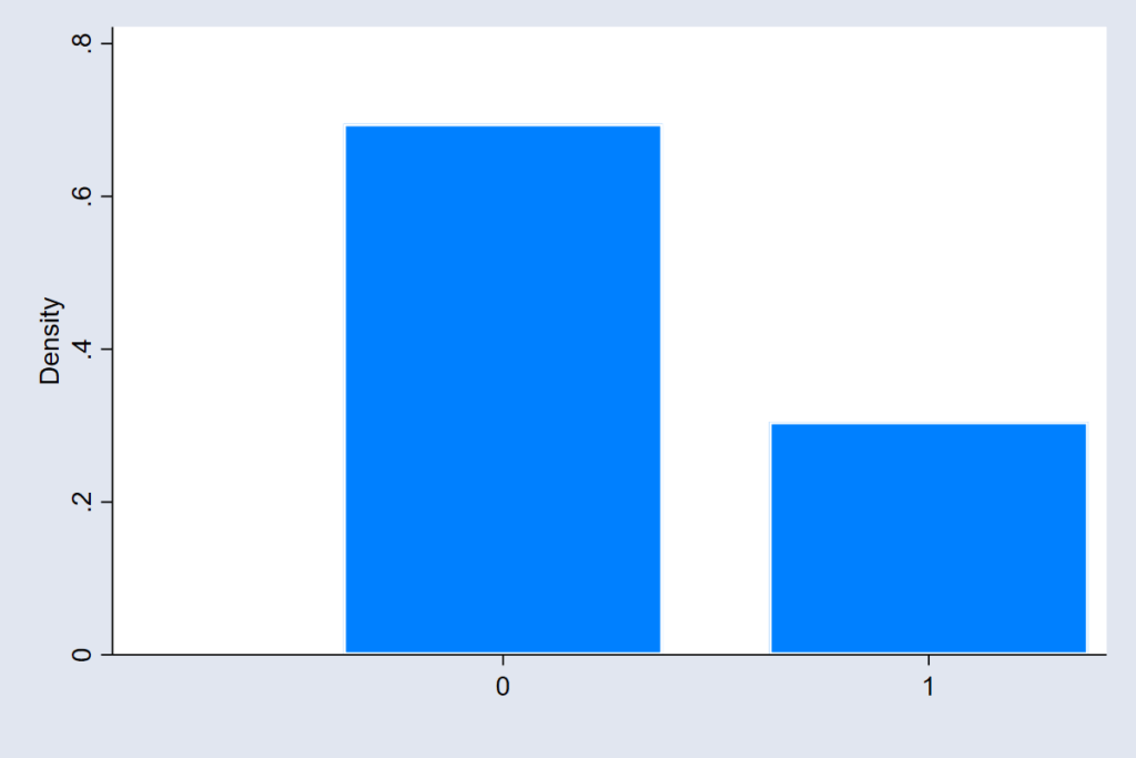
For settings where outcomes are binary (yes or no), the model assumes an underlying Bernoulli distribution. Here, randomness doesn’t vary continuously; it flips between two possibilities (see figure 3). The model’s uncertainty isn’t about how far off the mark it might be, but about which side of the threshold reality will land on—like predicting whether a citizen will vote or a client will default.
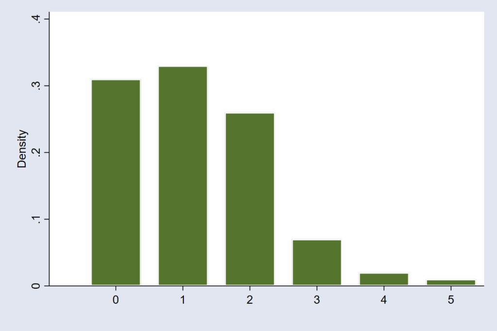
And when the model deals with counts — the number of hospital visits, crimes, or accidents per hour — the error structure follows the Poisson distribution. This distribution imagines that random events happen independently but at an average rate. It handles the fact that count data are whole numbers and can’t be negative (see figure 4).
Each of these distributions tells a different story about uncertainty — not in the outcome itself, but in the errors that remain after the model does its best to explain the world. Yet, in practice, many people look at the shape of the outcome variable — say, by drawing a histogram — and assume that is what matters for checking normality. But is it? The real question is whether the unexplained part of the model follows the assumed pattern. It is a subtle but powerful shift in thinking — one that changes how we judge whether our model truly fits the world it is meant to describe.
What is the Policy Cost of Assuming Wrong Distribution?
In practice, the choice of error distribution shapes how we judge whether an effect is real, how confident we are in it, and how we interpret uncertainty around it. When this fundamental assumption about the “noise” is wrong, even the most carefully estimated regression coefficients can give a false sense of precision. Three types of mistakes are especially common.
The first is mistaking noise for a signal. Statistical significance — the much-quoted p-value — is based on how extreme the observed result is relative to the assumed noise pattern. If we assume that noise is tightly clustered, as in a Normal distribution, even random fluctuations can appear unusually large. A policymaker may approve a costly new program, believing the positive effect is genuine, when it may have simply arisen from statistical luck. In essence, the policy “win” was just random noise dressed up as reliable evidence.
The second is false confidence. Confidence intervals are designed to capture the true range of likely outcomes. The assumed error distribution determines how wide or narrow that range appears. If the true errors are more spread out than the model assumes, the reported interval will be too tight. Imagine a ministry using a “precise” forecast of school enrollment to plan budgets, only to discover that actual student numbers fall well outside the predicted range. The analysis did not fail because the data were bad, but because the uncertainty was fundamentally underestimated. The model promised more certainty than reality could deliver.
The third is blindness to extremes. The Normal distribution assumes that extreme values are rare. But in many policy settings — from financial shocks to disease outbreaks — extreme events occur more often than that assumption allows. These are known as “heavy-tailed” situations. When models ignore them, decision-makers underestimate how frequently the unlikely can happen. It is not the average year that tests a policy; it is the catastrophic bad year that wasn’t expected. Failing to account for this distribution means you are blind to the most critical risks facing your organization or population.
Each of these problems stems from the same root: assuming a pattern of randomness that does not match the world we are studying. The distributional assumption does not just affect technical details in a regression table; it defines the credibility of every conclusion drawn from it.
Conclusion
If the functional form (the Signal) tells us our best guess about a policy’s effect, the distribution assumption (the Noise) tells us exactly how much we can trust that guess. Both matters equally. Getting the shape of the effect wrong leads us to the wrong answer; getting the shape of the uncertainty wrong makes us falsely confident in the wrong answer.
For policymakers and practitioners, this means asking not only “What is the estimated impact?” but also “How reliable is it?” Behind every table of regression results lies an assumption about how noisy, unpredictable, or uneven the world is.
So, the next time you read a regression table or a research paper, go one question deeper. Do not settle for the coefficient alone. Ask: “Which distribution did the study assume for the errors, and what is the policy cost if that assumption is wrong?” Better decisions begin with more informed questions, especially about the noise we choose to ignore. By understanding the stochastic component, we trade false certainty for credible risk management.