Did you know that countries with higher rates of internet penetration tend to have longer lifespans? Or that nations with larger militaries often have healthier populations? At first glance, these patterns might seem logical. After all, internet access could improve healthcare access, and a strong military might indicate a stable government. But does this mean one causes the other? Or are we mistaking correlation for causation? Statements like “increased internet access leads to longer lifespans” are common in research and policy discussions. But, how can we be sure that this is a cause-and-effect relationship rather than just a coincidence?
In this blog, we will explore this issue using real-world data scraped from Wikipedia. We will analyse three interesting relationships involving life expectancy vs. internet penetration, state fragility, and military size. Through this analysis, we will discuss the hidden pitfalls of assuming correlation equals causation. Along the way, we will also walk through the Python code used for web scraping and analysis. Whether you are a coding enthusiast or just curious about the findings, you can follow these codes along at your own pace.
Web Scraping for Research and Practice
Web scraping empowers researchers and policymakers by providing access to a wealth of data that might otherwise be unavailable or difficult to obtain. It automates the extraction of data directly from online sources, allowing researchers to create customised datasets tailored to their specific research questions. Decision-makers can use web scraping to track progress on policy goals, monitor interventions, or identify emerging challenges as they unfold. The ability to gather and structure data in an automated way not only saves time but also makes large-scale, real-time analysis possible, something that would be nearly impossible through manual data collection. However, scraped data often requires extensive cleaning due to formatting inconsistencies and missing values. Ethical considerations are also crucial, as some websites restrict automated access. To ensure responsible scraping, it is important to check a website’s robots.txt file and prioritise APIs when available for structured and ethical data access.
# Import necessary libraries
import pandas as pd
import numpy as np
import matplotlib.pyplot as plt
import matplotlib.lines as mlines
from bs4 import BeautifulSoup # Parse HTML and XML documents
import requests # Make HTTP requests to fetch web content
import seaborn as sns # Build statistical graphics on top of Matplotlib
import statsmodels.api as sm # For statistical modelling and inference
To illustrate the basics of web scraping, let’s extract country-level internet penetration data from Wikipedia. We first fetch the webpage using the requests library. Next, we employ BeautifulSoup to parse the HTML and locate the relevant data containing internet penetration rates. Once the data is extracted, we organise it into a structured format using the pandas library. This process follows the same logic for extracting other country-level indicators such as life expectancy, fragility index, and military size. Instead of repeating each steps in detail, I have prepared a cleaned dataset (wikidata.csv) that you can download and use directly. This allows us to focus on the analysis rather than spending time on pre-processing. Note that wikidata.csv contains data for LMICs only. High-income countries are excluded due to their significantly different socioeconomic and development portfolio.
# Scrap Internet Penetration Data from Wikipedia
net_url = "https://en.wikipedia.org/wiki/List_of_countries_by_number_of_Internet_users"
net_page = requests.get(net_url)
net_soup = BeautifulSoup(net_page.text, 'html')
net_table = net_soup.find_all('table', class_ = 'wikitable')[2]
heads = net_table.find_all('th')
table_heads = [head.text.strip() for head in heads]
inet = pd.DataFrame(columns=table_heads)
net_data = net_table.find_all('tr')
for row in net_data[2:]:
    row_data = row.find_all('td')
    country = [data.text.strip() for data in row_data]
    length = len(inet)
    inet.loc[length] = country

inet = inet.drop(columns = ['Rate(WB)', 'Year', 'Users(CIA)', 'Notes'])
inet.rename(columns = {'Location': 'Country', 'Rate(ITU)': 'Internet'}, inplace = True)
From Data to Correlation
Now that we have extracted and cleaned our dataset, we can move on to analysis. In this section, we examine how internet penetration, state fragility, and military size relate to life expectancy. First, we fit a linear regression model using the statsmodels library and visualise these relationships in scatter plots. The same approach applies to all three variables.
# Remove missing values
wikidata = pd.read_csv("wikidata.csv")
subdf = wikidata[['code', 'lexp', 'inet']].dropna()

# Fit a linear regression
X = sm.add_constant(subdf['inet'])  # Add intercept
y = subdf['lexp']
model = sm.OLS(y, X).fit()
slope = model.params['inet']  # Extract the beta coefficient
intercept = model.params['const']

# Create Scatter plot
fig, ax = plt.subplots(figsize=(8, 6))
sns.scatterplot(x='inet', y='lexp', data=subdf, color='dodgerblue', s=20, alpha=1)

# Add Regression line
sns.regplot(x='inet', y='lexp', data=subdf, scatter=False, color='red', ci=None, line_kws={'linewidth': 1})

# Display intercept and slope in the plot
eqn_text = f"Intercept = {intercept:.2f}, Slope = {slope:.2f}"
ax.text(0.05, 0.95, eqn_text, transform=ax.transAxes, fontsize=12, color='black')

# Set aesthetics
ax.set_xlabel("Internet Penetration Rate (%)", fontsize = 12)
ax.set_ylabel("Life Expectancy at Birth (Years)", fontsize = 12)

# Turn off the frame
ax.spines['top'].set_visible(False)
ax.spines['right'].set_visible(False)
plt.savefig("fig1.jpeg", dpi=150, bbox_inches='tight')
plt.show()
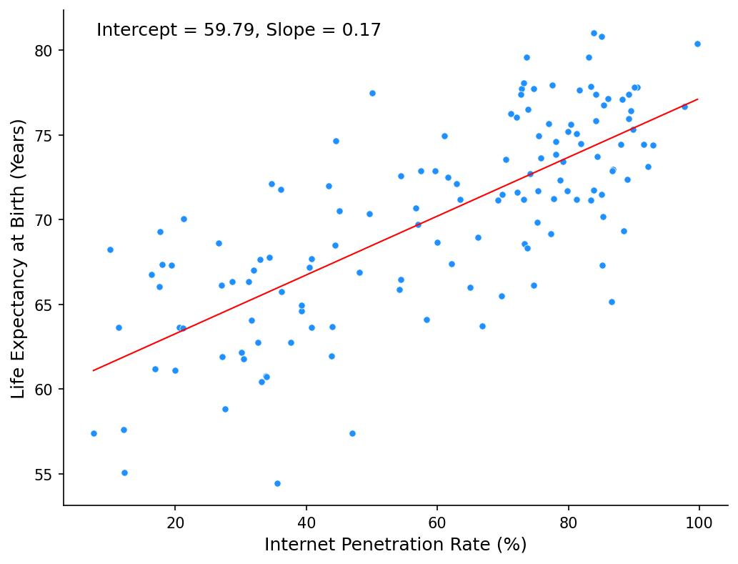
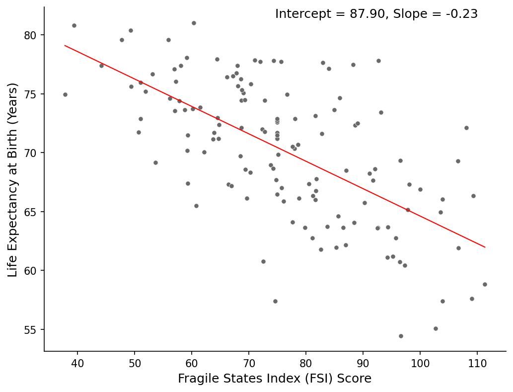
Figure 1 shows that for every 1% increase in internet penetration, life expectancy is predicted to rise by 0.17 years. The intercept (59.79) suggests that in a hypothetical scenario where a country has zero internet access, life expectancy would be almost 60 years. However, since a complete lack of internet is rare today, this intercept is more of a mathematical construct than a meaningful real-world estimate. Figure 2 suggests that countries with higher levels of state fragility tend to have lower life expectancies.
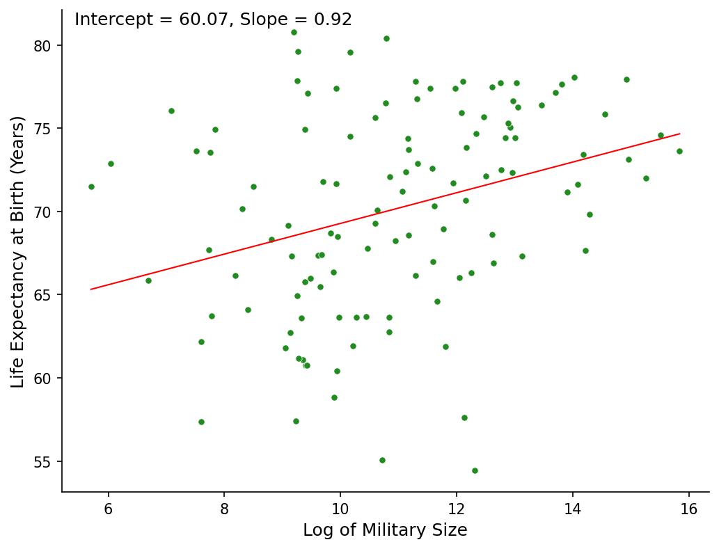
Figure 3 indicates that countries with larger militaries (in log terms) tend to have higher life expectancies. Using the log of military size means that the slope captures proportional changes rather than absolute increases in personnel. As a result, interpreting the relationship in terms of direct changes in military size becomes less intuitive. This highlights the importance of choosing appropriate transformations in regression models. If we had used a square or square root transformation, or even a different logarithmic base, how might our interpretation change? More broadly, what factors guide the choice of transformations—variable distributions, model fit, or the interpretability of coefficients? Take a moment to reflect on these issues in your research context.


Correlation vs Causation
Observing the three figures from the previous section, you might have noticed apparent relationships between internet penetration, military size, and state fragility, each with life expectancy. However, does a higher internet penetration rate necessarily cause people to live longer? Do fragile states inherently reduce life expectancy? Or does expanding a country’s military improve public health? This brings us to three common pitfalls of correlation.
It is crucial to remember that correlation does not imply causation. Our analysis highlights three key pitfalls that can lead to misleading interpretations of the observed relationships. First, confounding occurs when an unobserved factor influences both variables, creating a spurious association. Wealthier countries tend to have both higher internet penetration and better healthcare systems, making it unclear whether internet access directly contributes to longer life expectancy or if both are simply linked to broader economic development (figure 1). Second, the common cause problem arises when two variables share an underlying driver. The negative correlation between state fragility and life expectancy does not necessarily mean fragility directly shortens lives; rather, both may be shaped by weak governance, poor healthcare infrastructure, and economic instability (figure 2). Finally, reverse causality challenges the assumption that one variable influence another when the opposite may be true. While our analysis suggests a positive association between military size and life expectancy, it is more likely that wealthier, more stable nations—where people already live longer—can afford larger militaries, rather than military expansion leading to increased life expectancy (figure 3).
Understanding causality requires more than just identifying correlations; it demands isolating the true effect of one variable on another. A relationship between two variables, such as internet access and life expectancy, can only be considered causal if we can isolate all other factors—both observed and unobserved—that might influence either variable. In other words, we need to ensure that any change in life expectancy is solely due to changes in internet access, rather than confounding factors like economic development or reverse causality, where longer life expectancy might lead to greater internet access. This is where counterfactual reasoning comes into play. The key question in causal inference is: what would have happened to life expectancy if internet access had been different, while everything else remained the same? Since we can never observe both realities for the same country at the same time, causal analysis relies on methods designed to approximate this counterfactual world. While this blog focuses on correlation, in future discussions, we will explore how researchers attempt to uncover true causal relationships using counterfactual reasoning.
Closing Remarks
Misinterpreting correlation as causation can have serious consequences for development policies and interventions. In development research, correlations often reveal important patterns, but without understanding the underlying factors driving these relationships, policies based on such findings may fail to achieve their intended impact. So, effective communication of research findings is crucial, as the language used can significantly influence how these findings are interpreted and applied. Terms like “impact“, “effect“, and “leads to” are frequently used in development reports and media (and often in research papers) without careful consideration of causal mechanisms, blurring the line between association and true influence. This can mislead policymakers and the public.
In an increasingly data-driven world, the ability to distinguish between correlation and causation is more than just a technical skill; it is essential for responsible decision-making. As we grapple with complex global challenges, the questions we ask and the methods we employ will determine whether our insights drive meaningful change or perpetuate misconceptions. By recognising the limitations of correlation and pursuing robust causal inference methods, we can ensure that our research and policy decisions are evidence-based and contribute to a better future.